I’m assuming y’all know about means. In my home school district mean, median, and mode were all taught in third or fourth grade and referenced occasionally in math classes subsequently. But I’m guessing you don’t know about types of means.
See, the mean we’re familiar with is more properly called the “arithmetic mean,” so called because it uses simple arithmetic. But there are others that show up in statistics and other scientific applications. The most common are the geometric mean, the harmonic mean, and the quadratic mean (also often called the root mean square). And all of these are based on the generalized f-mean.
A note before we start: in all of these examples, I’m going to use the data set {7, 9, 29, 40, 42, 42, 65,
70, 87, 89}, which has an arithmetic mean of 48.
Harmonic mean
The harmonic mean is actually pretty simple: it’s the inverse of the average of the inverses of your data. In mathematical notation, that’s

So let’s do an example. The first thing you do is find the inverse (


Quadratic mean
The quadratic mean (or root mean square) is likewise fairly simple; the only difference is that you square rather than inversing the data, and square root the resulting average. So in mathematical notation, that’s

Example time again. First we square each of the items, which gives us {49, 81, 481, 1600, 1764, 1764, 4225, 4900, 7569, 7921}. Summing gives us 30354, and dividing by 10 gives us 
Geometric mean
The geometric mean is somewhat more difficult to calculate, but it’s probably my favorite. In middle school I independently “invented” it while I was bored in math class, but pretty quickly gave it up because it turned out to be too unwieldy to calculate.
Now, if you’re familiar with arithmetic, quadratic, and geometric growth (which you should be) you might be able to guess what the geometric mean is. If not, here’s a hint:

This graph shows arithmetic growth (


If you guessed that calculating the geometric mean involves multiplying your data together, you’re correct and win a prize**!
The mathematical notation for the geometric mean involves a symbol there’s a good chance you haven’t seen (I know I hadn’t until I learned about geometric means): 

![G=\sqrt[n]{\prod\limits_{i=1}^{n}x_i}=(\prod\limits_{i=1}^{n}x_i)^{\frac{1}{n}}](https://s0.wp.com/latex.php?latex=G%3D%5Csqrt%5Bn%5D%7B%5Cprod%5Climits_%7Bi%3D1%7D%5E%7Bn%7Dx_i%7D%3D%28%5Cprod%5Climits_%7Bi%3D1%7D%5E%7Bn%7Dx_i%29%5E%7B%5Cfrac%7B1%7D%7Bn%7D%7D&bg=ffffff&fg=555555&s=0&c=20201002)
So, we could calculate that as it is, by finding the product of our ten numbers (4,541,693,011,128,000, over 4½ quadrillion) and then the 10th root of that (36.789). Which is fine. But if we had any more numbers, my calculator would overflow, and sometimes you need to calculate the geometric mean of hundreds of numbers. To avoid having to use a computer with a googol bytes of memory, we take advantage of logarithms.
If you took pre-calculus with Mr. Kawamura, you might remember—will remember, considering how much he drilled it into our heads—that 

Which is a hell of a lot easier to calculate.
So let’s go back to our example data set. The natural logarithms of the items are {1.946, 2.197, 3.367, 3.689, 3.738, 3.738, 4.174, 4.248, 4.466, 4.489}. The sum of those is 36.052, which divided by 10 gives us 

By now it should be obvious that the means for this dataset are not the same. To review, we’ve got:
| Mean Type | Mean |
| Arithmetic | 48 |
| Harmonic | 24.186 |
| Quadratic | 55.42 |
| Geometric | 36.789 |
In other words, 
Generic f-mean
Now you may be seeing a pattern here. All of these different means follow basically the same form. This form is called the generic f-mean. It can be described thusly:
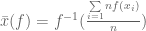
The only real restriction on this is that f be an invertible function. So you could go wild with this. You could use 


I’m not really sure what to write in conclusion, other than “means are cool!” so I’ll just leave it here. In a while I’ll come back to this topic. Coming up Wednesday, though, is a post on sample sizes and why (some) psychologists are stupid.
*Incidentally, were you to do this by hand and round as I did to the thousandth place, the math doesn’t add up exactly because of rounding errors.
**1.0 cookies****, redeemable by mail!
***You can actually use any base you want for the logarithm, since we’ll be reversing it. I just use ln since I’m a biology geek and e turns up a lot more than 10.
****With a 95% margin of error of 2.0 cookies.
Resources
Random.org Where I got the example dataset.
Mean at Wikipedia
Statistics Calculators Includes calculators for all of the means (other than the generic f-mean) that I discussed here.

